Detecting Patterns of Topological Signal Using Bipartition Covariance Networks
When looking for patterns in topological signals between competing phylogenetic hypotheses, one extremely helpful tool is bipartition covariance networks. By breaking each tree within a set down into its consituent bipartitions, or splits, statistical covariance analyses can be run in order to determine how specific bipartitions co-occur throughout a set of trees. For example, if a dataset contains trees generated using two different models of sequence evolution, one model may produce distinct, or even conflicting, topologies. In this scenario, bipartitions from trees generated using the same model would postively covary, meaning that they occur in the same tree often. Conversely, bipartitions that differ or conflict between trees generated using different models would negatively covary, meaning that they rarely occur in the same tree. Using bipartition covariance analyses and their accompanying visualization, these topological differences between trees can be readily identified and investigated in order to determine how trees differ down to the individual bipartitions.
1. Computing the Covariance Network
To perform a bipartition covariance analysis within CloudForest, all you need is an input set of trees, whether those trees come from inference using the Cipres REST API within CloudForest (details on that process here) or from an outside source.
Once the trees are input into CloudForest:
- Expand the CloudForest header in the tool panel on the left hand side of the screen
- Select the TreeScaper-Trees tool
- Under Output Type, select Covariance
- Indicate whether you want the trees to be interpreted as weighted or unweighted, and indicate if they are rooted or unrooted in the appropriate dropdowns
- Scroll down and select Execute to run the analysis

2. Visualize the Results
Once the analysis has completed, indicated by green items in the History panel, it’s time to visualize the results of the bipartition covariance analysis!
Note: In order to visualize results, you must be logged in to the platform. In order to log in select Login or Register at the top of the page, and for beta purposes, login using login/pw admin/admin
To visualize the results:
- Select visualize at the top of the screen, and select Create Visualization
- Scroll down to and select CloudForest Visualizations, and select Create Visualization
- Select Full Screen at the top of the page
- Under Visualization, select Covariance Plotting
- Under Files, select the relevant files to your analysis for Covariance Matrix, Bipartition Matrix, Bipartition Counts, Taxa IDs, and Tree File
- Select the green Run button to generate the visualization
3. Interpreting the Results
Using the visualization, you can view which bipartitions positively or negatively covary with others, as well as locate those bipartitions in trees visualized alongside the network. Branches can be hovered over with the cursor in the trees in order to highlight the corresponding bipartition node in the network, or bipartition nodes in the network can be hovered over with the cursor to highlight the corresponding branch in the tree. Bipartitions can also be selected with a mouseclick using the same methods in order to keep that bipartition highlighted on both plots, and multiple nodes can be selected with shift-clicking. Node(s) remain selected when scrolling through the treeset, enabling you to easily find where bipartitions occur within the treeset.

As pictured above, positive covariances are displayed as blue lines connecting bipartitions, and negative covariances red lines, with the strength of the covariance represented by the opacity of the line. Additionally, the frequency with which a bipartition occurs within the input treeset is reflected in the size and color of nodes in the network, with darker, larger nodes representing more common bipartitions.
Covariances, both positive and negative, are hidden if they do not exceed a threshold defined by the user using the Hide edges below X% of maximum input field. In addition, the Hide nodes with no edges above threshold checkbox will hide bipartition nodes in the network if they do not have covariance over the user-defined threshold. Finally, if the input treeset contains branch lengths, the Normalize branch lengths checkbox allows the user to toggle between displaying the trees as Cladograms or Phylograms.
Using the Bipartition Covariance tool and the accompanying visualization within CloudForest allows for extremely customizable and focused analysis of phylogenomic datasets in a way that few other methods allow. Community Detection analyses, also available within CloudForest, can also be performed on the bipartition covariance networks in order to detect natural groupings of bipartitions in the network. These results can be overlayed on top of the results shown here, similar to that done with NLDR results in the Community Detection tutorial. Stay tuned for a future tutorial where we detail the computation and visualization of community detection results using bipartition-covariance networks!
